How to optimise Julia code: A practical guide
Written 2022-06-08
You only have to spend a few minutes on a Julia forum to notice that its users really, really care about performance. If you have some Julia code you would like to be faster, simply post your snippet on Discourse and claim that 'Julia's speed is overrated', and 'It's no faster than Python', then you can find a lightning fast version of your snippet when you revisit the thread.
Unfortunately, that approach doesn't really scale. For any real project, you have to do the performance tuning yourself.
But how? In those Julia threads, one stumbles across a wide variety of optimisation issues, and a correspondingly diverse set of tooling to cast light on them. I imagine that for a newbie faced with performance problems, it can be disorienting. Where do you even begin?
Given that Julians are a flock of performance-obsessed academics, there are surprisingly few tutorials out there on optimisation of Julia code[1]. So I thought I'd write one, and this is it.
It's written for Julia 1.7.3. It is possible in the future the tooling around the language will improve such that some advice here becomes outdated. If so, write me a mail and I'll update this post!
Preface
Prerequisites: What to learn first
You can't write fast code without knowing a few basics on how computers, algorithms, and Julia work - quite a few basics, actually. You should:
If you are unfamiliar with hardware concepts such as CPU caches, memory alignment, or using SIMD instructions, please first read my guide on computer hardware. Preferably, you should also learn all the prerequisites of that namely,
Basics concepts in algorithms like big-O notation
How integers and floats are represented in memory
The memory layout of strings and their encoding
The layout of
Arrays, and the difference between inline arrays and arrays of pointersCommon data structures like hash tables
Have a grasp on some Julia basics: What type stability and inferrability is, and have at least a little experience writing and running Julia code.
You should read the official Julia performance tips.
Learn when not to optimise
Before you start optimising, make sure you actually need to.
This advice may seem so trivial it is vacuous, but unfortunately, needless optimisation is common in software. While speed is a quality of good code, the process of code optimisation often sacrifices other desirable aspects: Optimised code is often more verbose, and less readable, future-proof, testable or portable. Hence, when you needlessly optimise code, you may be spending your time actively degrading your code's overall quality.
In particular, be vigilant of the human tendency to categorise in binary absolutes: It is easy to think of computer operations as either "fast" or "slow". When it comes to code performance, these labels are meaningless without a point of reference. CPUs can do a billion operations in the time it takes a human to blink. That is so fast our human intuitions of "slow" and "fast" break down:
A ten nanosecond operation may be considered slow compared to arithmetic functions like multiplication, but is insignificant compared to a one microsecond syscall. Conversely, a one microsecond syscall is immaterial compared to a one millisecond file read, which is still imperceptibly fast on a human scale. Because "slow operations" can still be plenty fast on the scale that matters, any absolute categorisation of code patterns as "slow" or "fast" will mislead you.
Lastly, be aware that the contents of this post are rules of thumb. Any particular advice on how to optimise a piece of code is like advice on how to fix your car: Whether or not it is useful to you depends a whole lot on what the problem was in the first place. What I can offer here is a good default workflow for finding and eliminating inefficiencies - but of course I can't predict which inefficiencies cause your code to run slow, so you need to apply your knowledge to your own code's particularities.
Tools
Before giving workflow recommendations, it's useful to first introduce the different tools you have at your disposal. The how-to guide further down the post is laid out as a fixed list of instructions to follow when optimising code, but it is better used as only a loose guideline. To work effectively, you need to be able to reach for the right tool at the right time.
@time
The @time macro and its verbose cousin @timev are some of the simplest, yet most useful tools in your toolbox. Running @time will evaluate the following expression, and print the elapsed time. It will also report estimates of compilation time, garbage collection time, and the number and size of allocations.
This macro is most useful when a rough estimate is good enough. Because it simply uses a timer, its inaccuracy makes it unsuitable for code that takes less than about one millisecond to run.
BenchmarkTools
When @time is too inaccurate, particularly for small, fast functions, the similar macros @btime and @benchmark, provided by the BenchmarkTools package, come in handy. When typing e.g. @btime 1+1, the macro creates a closure () -> 1+1, then evaluates this repeatedly in a loop. It then prints the minimum runtime and number of allocated bytes:
julia> @btime join(['a', 'b', 'c'])
  232.712 ns (4 allocations: 240 bytes)
"abc"
The idea behind printing the minimum run time is as follows: It is assumed that the code has a fixed runtime in an idealised setting, but that this runtime is randomly prolonged by other programs interrupting your program's execution. Under this model, the minimum time is the least biased estimate, and closest to the true runtime.
Obviously, this assumption is sometimes wrong. For example, the function could have varying runtime, e.g. in the case of linearly searching a vector whose content is randomized between each run. In this case, the mean or the median runtime may be more informative, and the @benchmark macro should be used instead. This macro reports more statistics about the running time, and even prints a histogram of timings:
julia> @benchmark findfirst(isequal(100), x) setup=(x = shuffle!(collect(1:1000)))
BenchmarkTools.Trial: 8760 samples with 1000 evaluations.
 Range (min … max):    2.865 ns …   1.471 μs  ┊ GC (min … max): 0.00% … 0.00%
 Time  (median):     542.597 ns               ┊ GC (median):    0.00%
 Time  (mean ± σ):   551.176 ns ± 322.018 ns  ┊ GC (mean ± σ):  0.00% ± 0.00%

  █▆▄▄ ▄▄▅▆▅▅▃▆▅▅▅▄▅▄▃▄▆█▄▄▅▆▄▅▃▆▃▆▂▃▄▅▄▄▄▄▄▃▄▄▄▅▄▅▃▄▄▅▄
  ████▄█████████████████████████████████████████████████▆▄▄▃▃▃▃ ▇
  2.86 ns          Histogram: frequency by time          1.2 μs <

 Memory estimate: 0 bytes, allocs estimate: 0.
It's not always clear when a function has deterministic running time, and if you mistakenly think so, the minimum time can be horribly misleading. Therefore, I recommend just always using @benchmark and looking at the median and mean time instead of @btime.
Common BenchmarkTools pitfalls
Be careful not to use global variables when benchmarking. Not using non-constant global variables in performance-sensitive code is the number one Julia performance tip, but it is easy to accidentally copy-paste the content of a function into the REPL for benchmarking, thereby defining the function's local variables in global scope.
Another issue is that, because BenchmarkTools' macros create and run a closure, the benchmarking is vulnerable to being defeated by the optimising compiler, which may optimise away all the work. For example, here:
julia> @btime sin(55.1)
  0.030 ns (0 allocations: 0 bytes)
-0.9925515720731387
It reports a 30 picosecond runtime for sin. That would imply it takes 1/10th CPU cycle, which is clearly absurd.
What's happening is that the compiler used constant propagation and evaluated the result at compile time. The actual code being timed was:
julia> @code_typed (() -> sin(55.1))()
CodeInfo(
1 ─     return -0.9925515720731387
) => Float64
Which is instantaneous. You should see the BenchmarkTools documentation for how to handle these cases. This particular case can be handled by interpolating the value in using $:
julia> @btime sin($55.1)
  9.807 ns (0 allocations: 0 bytes)
-0.9925515720731387
The particular issue should be fixed when using BenchmarkTools with the upcoming version 1.8 release of Julia. But in general, the interplay between the compiler and BenchmarkTools is tricky and subject to change over time, and takes some effort getting the hang of the common pitfalls. If in doubt, you can always ask in a Julia forum or chat.
A more fundamental problem with using BenchmarkTools is that modern CPUs have various components that analyse and adapt to code on a hardware level, while it is running:
Data and instructions are cached for fast repeated access
Branches are being predicted, enabling speculative execution
Memory is being prefetched when an access pattern is detected
For more information on these, see my hardware introduction post.
Because BenchmarkTools run their closures repeatedly in a tight loop, the CPU is able to adapt extraordinarily well to the code compared to what it would be able to when executing your code in a realistic setting. As a result, the true running time is often quite significantly underestimated.
The branch predictor can be thwarted by benchmarking a larger example with millions of branches, but larger examples will not necessarily reflect the branching pattern of your code in the wild. Unfortunately, I don't know of any good way to get around these biases, or to detect if they skew your measurements.
@code_warntype
The @code_warntype macro is used to check if some code is inferrible. Like other code introspection macros, you put it in front of a function call:
julia> @code_warntype first(Any[1])
MethodInstance for first(::Vector{Any})
  from first(a::AbstractArray) in Base at abstractarray.jl:398
Arguments
  #self#::Core.Const(first)
  a::Vector{Any}
Body::Any
1 ─ %1 = Base.eachindex(a)::Base.OneTo{Int64}
│   %2 = Base.first(%1)::Core.Const(1)
│   %3 = Base.getindex(a, %2)::Any
└──      return %3
From top to bottom, it displays three pieces of information: First, which method instance was called. Hopefully you already knew this - if you don't know what code you are running, you are going to have a hard time optimising it! Second, the arguments, with #self# signifying the function. Again, the content here should not be surprising.
The third part is the lowered code - Julia's compiler operates code using different representations with varying levels of abstraction. After the raw source code, the lowered code is the highest level representation. I can heartily recommend any Julians to learn how to read lowered code (it's designed to be a simplified version of source code, so it's not that hard!) - but let's skip that now.
Each local variable is denoted by the % sign, e.g. %1 = Base.eachindex(a), and denoted with the type that the compiler is able to infer for the variable - in that case Base.OneTo{Int64}. The return variable is referred to as Body, and is placed above the lowered code.
When displaying the @code_warntype output in REPL, but unfortunately not on this blog, fully inferred (concrete) variables are coloured cyan, and abstract types are coloured red. In the example above, the result of the getindex call infers to Any, an abstract type, and is thus coloured red when shown in the REPL.
When optimising code, the crucial part is to look for the presence of these red coloured abstractly inferred variables which are detrimental to performance.
Other non-concrete types are coloured in yellow, for example the Union{Nothing, Int64} in:
julia> @code_warntype findfirst(isodd, [])
MethodInstance for findfirst(::typeof(isodd), ::Vector{Any})
  from findfirst(testf::Function, A::Union{AbstractString, AbstractArray}) in Base at array.jl:2002
Arguments
  #self#::Core.Const(findfirst)
  testf::Core.Const(isodd)
  A::Vector{Any}
Body::Union{Nothing, Int64}
1 ─ %1 = Base.keys(A)::LinearIndices{1, Tuple{Base.OneTo{Int64}}}
│   %2 = Base.first(%1)::Core.Const(1)
│   %3 = Base.findnext(testf, A, %2)::Union{Nothing, Int64}
└──      return %3
The idea is that the compiler is still able to generate efficient code for small unions of e.g. 2-3 concrete types, so this is not a concern for inference or performance.
JET.jl
JET is an amazing package which hooks into the Julia compiler and leverages it to do static analysis. It's relatively new, so it's possible the capabilities I illustrate here may be outdated in the near future.
In this context, the relevant functionality is JET's optimisation analysis. The @report_opt macro is analogous to recursively calling @code_warntype down the chain of all function calls, and printing areas of the code where type instability is detected:
julia> @report_opt foldl(+, Any[], init=0)
═════ 2 possible errors found ═════
┌ @ reduce.jl:180 Base.#foldl#245(kw..., _3, op, itr)
│┌ @ reduce.jl:180 Core.kwfunc(Base.mapfoldl)(Base.merge(Base.NamedTuple(), kw), Base.mapfoldl, Base.identity, op, itr)
││┌ @ reduce.jl:162 Base.#mapfoldl#244(init, _3, f, op, itr)
│││┌ @ reduce.jl:162 Base.mapfoldl_impl(f, op, init, itr)
││││┌ @ reduce.jl:44 Base.foldl_impl(op′, nt, itr′)
│││││┌ @ reduce.jl:48 v = Base._foldl_impl(op, nt, itr)
││││││┌ @ reduce.jl:81 +(init, %16)
│││││││ runtime dispatch detected: +(init::Int64, %16::Any)
││││││└────────────────
││││││┌ @ reduce.jl:62 op(%22, %41)
│││││││ runtime dispatch detected: op::Base.BottomRF{typeof(+)}(%22::Any, %41::Any)
││││││└────────────────@@
JET operates statically on a type level, and is thus, not able to find all type instabilities in your code. If your code contains a function call that is not statically inferrible, JET will report dynamic dispatch at that function call, but since the compiler (and thus JET) cannot infer across dynamic dispatch, JET can't report on any problems on the "other side", and therefore cannot find problems downstream of that call.
This limitation is normally not a big deal because only reporting the first instance of inference problems in a call chain is usually sufficient to alert you of performance problems.
Cthulhu
Cthulhu is not only a Lovecraftian cosmic horror, but also a Julia package that allows the user to interactively explore type inference in their code, letting you step into function calls one at a time while displaying the compiler's information.
It's most easily used as a better, more featureful version of @code_warntype, but its rich features makes it better suited to debug truly nasty type instability issues.
Profiler
Julia comes with the stdlib package Profile which is simple, but effective. It works by running your code and intermittently (e.g. every millisecond) pausing execution, sifting through the call stack and tallying each method in the stack. When it has run for a few seconds, it thus has several thousand samples of which methods were being executed during the run. If e.g. 1/100th of call stack samples contained the function foo, you can assume that about 1/100th of running time was spent in foo.
This assumption is not precise because the finite number of stack samples cause sampling noise, but it is usually good enough. It is possible for code to exhibit some kind of temporal pattern that will bias the sampling - for example, if your code happen to call a particular function every millisecond, this function may end up in a huge number of samples just by virtue of its timing being correlated with the sampling frequency. I suspect that will happen very rarely, though.
When running the profiler, make sure the task you are profiling is representative of your workload. Say, for example, you have a program with two tasks where the first scales linearly with the input size, and the second scales quadratically. In that case whether you should spend your effort optimising the first or the second part depends a whole lot on the size of the inputs. You might profile with a small toy example and erroneously conclude that most time is spent in the first task.
VSCode Julia profiler
The stdlib profiler is useful on its own, but the Julia VSCode extension includes the @profview macro, which improves the profiler with some very useful capabilities:
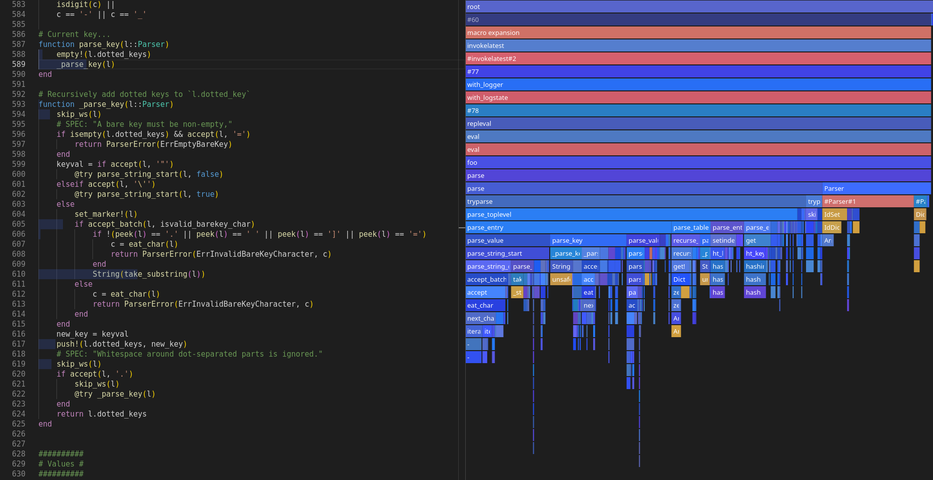
In the picture above, you see two panels: The code itself on the left, and the profiler results are displayed as a so-called flame graph on the right. Let's review the flame graph first.
Each of the coloured boxes represents a line of source code. They are labelled by the function the line occurs in. The one at the top represents the top-most function call. Since the VSCode profiler is called from the REPL, the first several boxes from the top stem from functions internal to the REPL and profiler. These have negligible overhead, and can usually be ignored - though make sure to not analyse your first call to @profiler, so you don't accidentally profile compilation of the profiling code itself.
The width of the box is proportional to the number of samples containing that line of code. A box placed below another means that the top box's function called the bottom box's function. If you mouse-over the boxes, it will show you which line of code is represented by the box. Clicking the box will open your editor at that line.
On the left side of the picture, in the source code, you can see some of the lines have been highlighted with coloured bars whose length are proportional to the number of samples that included that line.
The profiler gives one more piece of information: The color of the boxes (and code line highlights). Red lines mean dynamic dispatch (i.e. type instability) happened at that line. Yellow means the garbage collector kicked in, which happens during memory allocations.
Walkthrough: How to optimise
Now armed with knowledge of the available tooling, you can get started on your optimisation quest. Below I have written a list of things to try, in the order I recommend them.
Ensure your code is type stable
Type unstable Julia code is slow Julia code[2]. Indeed, the first tip of the Julia performance tips is to put code in functions instead of the global scope, so that it can be type stable. In fact, most of the official performance tips pertain to type stability.
Not only is type stable code faster, it is also better than unstable code:
Type stabilising your code often improve various aspects of code quality, in my experience. I'm not entirely sure why it is so - perhaps type stable code encourages small generic functions - or discourages type confusion.
Type stable code can be precompiled better and lead to fewer invalidations, reducing Julia's annoying compile-time latency.
Type stable code is statically analysable and enables tooling like JET to help you with your code. While static analysis is not yet ubiquitous in Julia, I find it likely that the future will see Julia linters backed by static analysis, presumably integrated into IDEs.
Newcomers to Julia have to pay attention when coding to write type stable code, but don't worry: It quickly becomes second nature. With experience, writing type stable code is effortless, and you develop an intuition of the rare occasions when you are writing a function that might be type unstable. In those situations, you can use @code_warntype to check your functions as you are writing them.
If you've written a larger chunk of code, and you don't feel confident you have caught all instances of type stability, you can run JET's optimisation analysis on some high-level function calls to check them and all their callees.
Profile your code
Type stability is as much about code quality as about performance - hence I view it more as a prerequisite for optimisation rather than optimisation itself. For real optimisation, the first step is always to figure out what to optimise.
Most code consists of a few small parts where most the time is being spent, and large parts which are unimportant to performance. Obviously, any time you spend optimising code that is not important for runtime is at best a waste of time, and at worst you are introducing bugs into working code for no gain.
In my experience, it's surprisingly difficult to predict which parts of your code are the former and which are the latter, even for programmers more experienced than I. So - before beginning real optimisation, measure your code, and only work on the parts that matter for performance. If you begin optimising before you measure, you are choosing to work while blind.
I recommend using the VSCode's profiler, which allows you to also pay attention to dynamic dispatch and allocations. If dynamic dispatch or allocations show up where you don't expect them to, that is an obvious place to look at.
Review your algorithms
The largest performance gains are reaped not from small tweaks, but from using the appropriate algorithms to solve your problem. Now that you know where to optimise, begin by reviewing your approach to the problem.
Take the 10 kilometre birds-eye view of your code and ask yourself:
How do the speed of my approach scale with input size? For this, you should think in terms of Big-O notation. That is, if the size of my input doubles, what does that imply for the running time of my code? Does it double? Quadruple? Even worse?
Can you approach the problem differently, or use any data structures that allows a better performance? Typical moves here may be to replace large vectors with sets for faster membership testing, or avoiding the creation of collections using multiple rounds of concatenation.
Is the code doing needless repeated work? Without going into details about exactly how the code is executed on a low level, does the code do stuff it doesn't need to that can be cut away? An example here may be code that runs a function
fon an array in a loop, wherefsorts the array first. In that case, you could refactor the sorting out offand put it before the loop.Have someone else already solved the problem for you in a good, reliable package? If so, just use it and don't sweat about re-inventing the wheel.
Cut down on allocations
Computation is generally faster than memory access on modern computers. Reducing allocations, therefore, is usually an easy performance win.
You can use the VSCode profiler to find where the GC is running (which implies memory is being allocated), or use Julia's memory allocation profiler.
Some tips to reduce allocations are:
Use immutable structs over
mutable structwhen mutation is not neededUse tuples or
StaticArrays instead of short arrays if the length and element type is known at compile timeUse substrings and array views where possible
Prefer lazy generators and iterables over materialized results
Preallocate buffers once and reuse them multiple times
The packages Setfield, StaticArrays, InlineStrings and StringViews can come in handy here.
Create types for efficient representation
It is often said that in Julia, abstraction is free in terms of performance. In my experience however, not only does abstraction cost nothing, it results in faster code, if you create your abstractions with performance in mind. This is primarily because abstraction allows you to carve out and isolate a part of the code, and then to optimise it to your heart's contend without it affecting the rest of the codebase.
Nowhere is this more effective than the creation of custom types with efficient memory layouts and methods specialized for your workloads.
As a case study, consider InlineStrings' type String31. It is an AbstractString that can hold any String of 31 code units or fewer - but it has the memory layout of a 256-bit integer, meaning it can be stored inline in arrays or in a single SIMD register. When dealing with large arrays of strings that are known to be a fixed size (e.g. identifiers), choosing String31 over String can make a massive performance difference.
Some other good examples of efficient custom types are:
Besides giving excellent performance, making your own types also gives better opportunities to enforce invariants of your data by putting them in the constructors and the interfaces of your new type.
A practical advice is to look through your code and see when you conceptually use a type whose structure is not perfectly captured by any existing types in your code. For example, if you see Vector{Tuple{String, UInt8, DNA}}, in your code, then it probably means you need to refactor the tuple out to a new struct, which you then can optimise.
Use multiple threads
If your task is easily parallelisable, you can make your code several times faster by using multiple threads. But beware: Introducing multithreading to a program opens a whole can of nasty concurrency bugs, and I would avoid doing it unless the extra speed is needed - hence why this advice is far down the list.
Multithreading is easiest (and usually most effective) to do on a coarse-grained level, on loops high up in the call chain. This is because thread spawning and management has some overhead.
A simple way to begin is to find the highest-level parallelisable for loop in your code (still only if your code actually spends time there, right?) and slap Threads.@threads on it.
If you are more comfortable with a functional style of programming, the package Folds.jl and the broader JuliaFolds ecosystem have types and functions that enable automatically parallelisable folds. For example, Folds.reduce(op, collection) works analogous to Base.reduce, but is parallel by default.
For more advanced uses, you can micromanage individual threads using the primitives in the Base submodule Threads. Messing around manually with threads is so error prone that I don't recommend doing this unless necessary for performance.
Reduce memory consumption
"Data-oriented design" (DoD) means designing your data structures - and by extension, your code - to optimise their memory footprint and data layout over other concerns. It is derived from the idea that computation is usually faster than memory access. For more details on this, see my hardware introduction.
There are a number of interesting talks on DoD I recommend watching, most famously Mike Acton's. Andrew Kelley gave another wonderful talk on DoD where he gives some concrete suggestions to reduce your data's memory footprint.
Unfortunately, the most efficient data layout is not necessarily the easiest to reason about, to read, or to refactor. Therefore, adopting DoD can come at the expense of other qualities of code, and thus should be considered an advanced performance trick to reach for only when performance is a top priority.
Practical tips for DoD generally boils down to two aspects: Work hard to have your structs use less memory, and group similar data together:
Do not store fields that can easily be computed on demand.
Reduce integer sizes from e.g.
InttoInt32orInt16where possible.Try not to store booleans: Either encode them into an unused bit of another field, or store them implicitly by grouping the structs by the value of the boolean.
Re-order fields of your struct to reduce padding (Julia uses same struct layout as C does)
Instead of storing 64 bit pointers to objects like
Stringin your structs, keep all these objects in an array and store the relevant index into the array, which may only take 32 or 16 bits.Data locality can be improved by switching from array-of-structs to struct-of-arrays. That is, instead of having a
Vector{Foo}whereFoois this:
struct Foo
	a::Int32
	b::UInt16
end
Store the same data like this:
struct FooArray
	as::Vector{Int32}
	bs::Vector{UInt16}
end
Review generated assembly
If your code spends most of its time in a few core functions, it can pay off to inspect the assembly code generated by these functions and micro-optimise them. I prefer reading the native code from @code_native because I find it more readable than the LLVM code generated by @code_llvm, but others prefer LLVM.
Some people think that having assembly code guide your optimisation is a terrible idea, because assembly is too far removed from idiomatic Julia. I disagree. Viewing assembly code can often be excellent for diagnosing issues with the overlying Julia code. These can then be fixed on a higher level, and the fix will show itself in improved assembly code. In my experience, the performance gain from micro-optimising assembly can be significant, even if you only ever write high level Julia.
A good place to start is to look for vectorisation. If you believe the code should vectorise, scan the assembly for the presence of vector instructions, which can be identified in x86 assembly by usually beginning with "vp". If there are no such instructions, find out what is inhibiting vectorisation and remove these barriers. It will typically be one of:
Boundschecks, which you can disable with
@inbounds(be careful)Non-associativity of operations. In particular float operations are usually not associative, but this only makes a difference by introducing tiny rounding errors that are fine in most contexts, so you can use
@simd.Branches inside the loop body that you might be able to refactor away
Next, look for instructions that seem out of place. Granted, it takes a little experience to get a feeling for what instructions are expected. I usually notice integer/floating conversion instructions and callq instructions, in particular to error throwing functions and to jl_box. If these kinds of needless instructions are there, you can typically simplify the code somewhere.
Finally, follow all the branches in the code and see if each of them makes sense. Branches are useful to look at because redundant work like needless error checks or type conversions often involve a branch. In a way, the execution flow of a function is summarised by the branching pattern. Branches can also directly slow your code down by causing branch mispredictions. Lastly, in my experience, LLVM is very, very good at optimising non-branch instructions, especially bitwise operators, but usually can't optimise away non-dead branches. Find any out-of-place branches, and simplify your code to remove them.
| [1] | As it turns out, there are actually quite a few already. I quickly discovered that when I shared this post with the broader Julia community: this and this and this and this and this and this and this and possibly several more I have missed. |
| [2] | Already here I violate the advice I gave in the preface: To not think of certain operations as inherently slow. Type instability causes dynamic dispatch, which typically take tens to hundreds of nanoseconds. There are plenty of contexts where a fraction of a microsecond is negligible. Use your judgement. |